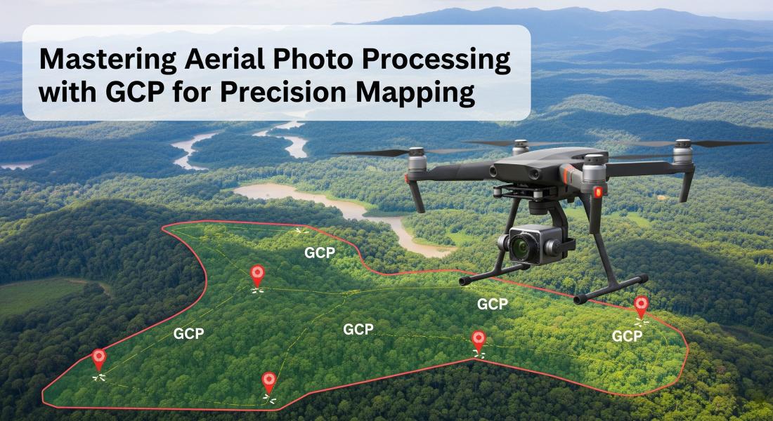
In the exciting world of drone technology and geospatial data, processing aerial photos efficiently and accurately is absolutely crucial. Whether you're mapping agricultural fields, conducting topographic surveys, or creating stunning 3D models of historical sites, the quality of your output heavily relies on precise photogrammetry. This is where software like Agisoft Metashape truly shines, especially when combined with the power of Ground Control Points (GCPs). This comprehensive guide will walk you through the process of mastering aerial photo processing using Agisoft Metashape, assuming your GCPs are already prepared and ready for action.

What are Ground Control Points (GCPs) and Why Are They Essential?

Before we dive into the "how-to," let's quickly recap why GCPs are your best friends in photogrammetry. Ground Control Points are precisely measured points on the ground with known geographic coordinates (latitude, longitude, and altitude). When you integrate these points into your photogrammetry workflow, they act as anchors, significantly improving the absolute accuracy and georeferencing of your resulting maps, orthomosaics, and 3D models.

While Metashape can generate pretty good models without GCPs (using only GPS data from the drone), GCPs are indispensable for achieving survey-grade accuracy, correcting for GPS drift, and ensuring your data aligns perfectly with real-world coordinates. For this tutorial, we're operating under the assumption that you already have your GCPs surveyed and their coordinate list ready to be imported.

Getting Started with Agisoft Metashape

Agisoft Metashape (formerly PhotoScan) is a powerful standalone software product that performs photogrammetric processing of digital images and generates 3D spatial data. Let’s open it up and get ready to process your drone imagery.

1. Creating a New Project

First things first, open Agisoft Metashape and start a new project. It’s always good practice to keep your projects organized.

Go to the File menu and select New.

2. Adding Your Aerial Photos

Now, let's load your drone images into the project. Make sure all your photos are in a single folder for easy access.

Go to Workflow > Add Photos... or simply click the "Add Photos" icon on the toolbar. Navigate to your image folder, select all your photos, and click Open.

You'll see your photos appear in the "Photos" pane. Each photo will have a little camera icon next to it.

3. Aligning Photos

The first major processing step in Metashape is photo alignment. This step identifies common points across your images and reconstructs the camera positions and orientations for each photo, creating a sparse point cloud.

Go to Workflow > Align Photos...

In the "Align Photos" dialog, you'll see several parameters:

• Accuracy: For most drone mapping projects, "High" or "Highest" is recommended. "Medium" can be used for quicker previews or less critical projects.
• Generic preselection: Keep this enabled for faster processing.
• Key point limit & Tie point limit: Default values are usually fine, but you can increase them for more challenging datasets (e.g., highly textured areas, sparse overlap).

Click OK. This process can take some time depending on the number of photos and your chosen accuracy. Once complete, you’ll see a sparse point cloud and the estimated camera positions in the 3D viewport.

Importing and Placing GCPs in Agisoft Metashape

This is the core of our tutorial. Having pre-prepared GCPs simplifies this step significantly, but precision is still paramount.

1. Preparing Your GCP List

Your GCP data should typically be in a text file (.txt or .csv) containing the GCP name and its X, Y, Z coordinates (Easting, Northing, Altitude or Latitude, Longitude, Altitude). Make sure you know the coordinate system of your GCPs!

A typical format might look like this:

Station	Latitude	Longitude	    Height
1	 -7.277641667	112.796933333	32.9115
2	 -7.279044444	112.795513889	34.3007
3	 -7.279894444	112.797941667	32.7445
4	 -7.280427778	112.796391667	32.991
5	 -7.281377778	112.792516667	32.7718
BNK1 -7.284216667	112.793158333	32.8219
FTK1 -7.281636111	112.797675000	32.6504
PPS1 -7.281869444	112.795261111	32.151
SCC1 -7.283338889	112.792994444	32.5466
TKM1 -7.283152778	112.795894444	32.3231

2. Import GCPs into Metashape

Go to the Reference pane (usually at the bottom left, if you don't see it, go to View > Panes > Reference). Right-click inside the Reference pane and select Import GCPs...

In the "Import CSV" dialog:

• File: Browse to your GCP file.
• Columns: Metashape will try to auto-detect, but ensure they are correctly mapped (e.g., Label, X, Y, Z).
• Coordinate System: This is CRITICAL. Select the exact coordinate system of your GCPs (e.g., WGS84, UTM Zone 10N, etc.). If you’re unsure, consult with whoever provided the GCP data.
• Delimiter: Set this to what your file uses (e.g., comma, tab).
• First Line is Header: Check this if your file has a header row.

Click OK. Your GCPs will now appear in the Reference pane.

3. Marking GCPs on Your Photos

This is the most critical and often time-consuming step for accuracy. You need to identify each GCP in at least 2-3 (preferably more, 5-10 or more for best results) photos where it's visible and mark its exact center.

In the Reference pane, Select one GCP in the reference tab. Then, right click on that GCP and select filter photos by marker. Metashape will display the photos that are likely to contain that GCP.

For each GCP:

1. Select the GCP in the Reference pane, Then, right click on that GCP and select filter photos by marker.
2. In the "Photos" pane, identify images where the GCP is clearly visible. Double-click on an image to open it in a larger viewer.
3. Zoom in closely on the GCP target in the photo.
4. Right-click and drag on the exact center of the GCP target and select Place Marker > [GCP Name].
5. Repeat this for as many images as possible for that GCP for all images. The more images with precise markers, the better the accuracy.
6. Once you have marked the GCP in a few photos, Metashape will often project the estimated position onto other photos as a small white circle. You can then fine-tune these projections by dragging the marker to the precise location. A red flag indicates a manually placed marker, while a blue flag indicates a projected marker.

Repeat this process for ALL your GCPs. Patience and precision here pay off immensely.

Once you’ve marked all your GCPs, you'll see green flags in the "Reference" pane indicating the points are ready.

After all GCPs are marked, it's time to perform optimized cameras. This step will recalculate and refine the internal and external camera parameters based on GCP data, resulting in smaller errors and higher accuracy.

4. Optimizing Camera Alignment

After marking GCPs, it's essential to optimize the camera alignment. This step refines the camera positions and orientations based on the newly introduced precise GCPs.

In the Reference pane, make sure your GCPs are enabled (checkbox next to them is ticked). Go to Workflow > Optimize Cameras...

In the "Optimize Cameras" dialog, you can leave the default parameters for now. Make sure "Adapt focal length," "Adapt principal point," and "Adapt radial distortion" are checked for best results. Click OK.

After optimization, check the "Error (m)" column in the Reference pane for your GCPs. These values represent the projection error for each GCP and should be as low as possible (ideally below 0.05m to 0.1m, depending on your target accuracy). If the error is too big, you can repeat the GCP process. It is possible that the GCP point is not in the middle of the GCP marking as it should be.

Building Your Products: Point Cloud, DEM, and Orthomosaic

1. Building Point Cloud

The point cloud is a highly detailed representation of the scene, generated from the sparse cloud and camera positions.

Go to Workflow > Build Point Cloud...

Parameters to consider:

• Quality: "High" or "Ultra High" for best results, but "Medium" or "Low" for faster processing or preview.
• Depth Filtering: "Aggressive" for noisy data, "Mild" for smooth surfaces, "Disabled" for maximum detail (at the risk of more noise).

Click OK. This is often the longest processing step.

2. Building Mesh and Texture Bringing Your Model to Life

The dense cloud is a collection of points. To create a solid, renderable 3D model, you need to build a mesh (a polygonal surface) and then apply textures from the original images.

Building the Mesh

1. Go to "Workflow" > "Build Mesh...".
2. Important settings:
   • Source data: Select "Dense Cloud".
   • Surface type: "Arbitrary" for most objects. "Height Field" is better for flat terrain where you want a DEM-like mesh.

   • Face count: Determines the polygon count of the mesh. Higher numbers mean more detail but larger file sizes and slower rendering.

     

3. Click "OK".

Building the Texture

1. Go to "Workflow" > "Build Texture...".
2. Key parameters:
   • Source data: "Images".
   • Mapping mode: "Generic" is good for most models.
   • Blending mode: "Mosaic" provides seamless blending of textures.

   • Texture size/count: Adjust based on desired resolution and target platform.

     

3. Click "OK". Your 3D model will now appear textured in the "Model" view.

3. Building DEM (Digital Elevation Model) or Tiled Model

A DEM is a raster representation of the terrain's elevation. An orthomosaic needs a DEM to be accurately projected.

Go to Workflow > Build DEM...

• Source Data: Usually "Dense Cloud."
• Interpolation: "Enabled" is generally recommended.
• Coordinate System: This should match your project's desired output coordinate system, typically the same as your GCPs.

Click OK.

4. Building Orthomosaic

The orthomosaic is a geometrically corrected, seamless image of your project area, free from distortions and scaled accurately.

Go to Workflow > Build Orthomosaic...

• Surface: Select "DEM" as the source.
• Blended Mode: "Mosaic" is standard for seamless blending.
• Pixel Size: Defines the ground sample distance (GSD) of your output. This should be set according to your project requirements.
• Coordinate System: Again, ensure this matches your desired output.

Click OK.

Exporting Your Results

Once processing is complete, you can export your orthomosaic, DEM, or 3D model.

• To export Orthomosaic: File > Export > Export Orthomosaic... (e.g., GeoTIFF)
• To export DEM: File > Export > Export DEM... (e.g., GeoTIFF)
• To export 3D model (if you built one): File > Export > Export Model... (e.g., OBJ, FBX)

Always double-check the export coordinate system and ensure it's correct for your downstream applications.

Tips for Success

• GCP Distribution: Ensure your GCPs are well-distributed throughout your project area, especially at the corners and in the middle. Do not cluster them in one spot.
• Image Quality and Overlap: High-resolution, sharp images with at least 70-80% frontal overlap and 60-70% side overlap are ideal for robust processing.
• Processing Settings: Don't always jump to "Highest" quality. Start with "High" and consider if "Ultra High" is truly necessary, as it significantly increases processing time and resource consumption.
• Check Reference Pane Errors: Always monitor the error values in the Reference pane after optimizing cameras. High errors might indicate incorrect GCP marking or erroneous GCP coordinates.
• Save Frequently: Photogrammetry can be resource-intensive. Save your project regularly to avoid losing progress.

Common Challenges and How to Overcome Them

Even with prepared GCPs, you might encounter a few bumps along the road. Here's how to navigate them:

1. Alignment Issues (Too Few Points, Cameras Not Aligned)

Problem: Your sparse cloud looks sparse, or many cameras failed to align.

Solution:

• Check Overlap: Ensure your drone flight plan had sufficient image overlap (70/60% minimum, 80/70% recommended).
• Image Quality: Verify photos aren't blurry, over/underexposed.
• Reprocess with Higher Accuracy: Try "Align Photos" with "High" or "Highest" accuracy and potentially increase "Key point limit" or "Tie point limit" in the advanced settings.
• Manual Tie Points: If a section consistently fails, manually add tie points between unaligned photos. Go to the "Reference" pane, select two unaligned photos, right-click, and choose “Align Selected Cameras.”

2. High GCP Residual Errors

Problem: After optimizing cameras, the "Error (m)" column for your GCPs shows values higher than acceptable (e.g., >0.1m or >0.2m).

Solution:

• Recheck GCP Marks: This is the most common culprit. Zoom in intensely on each GCP in every photo you've marked it in. Drag the marker precisely to the center of the target.
• Check GCP Coordinates: Double-verify the imported GCP coordinates against your source data. A single typo can throw everything off.
• Verify Coordinate System: Ensure the coordinate system you selected for importing GCPs (and for the project) exactly matches the coordinate system of your physical GCPs.
• Remove Bad Markers: If one specific photo consistently shows a very high error for a GCP, consider removing the marker for that photo.
• Redistribute GCPs: If errors are systematic across the project, your GCPs might not be optimally distributed. For future projects, ensure a good spread across the entire flight area.

3. Long Processing Times / Out of Memory Errors

Problem: Metashape takes forever to process or crashes with memory errors.

Solution:

• Lower Quality Settings: For initial runs or less critical projects, use "Medium" or "Low" quality for dense cloud and orthomosaic generation.
• Process in Chunks: For very large datasets, consider processing smaller sections of the project and then merging them.
• Upgrade Hardware: Photogrammetry is very demanding. More RAM, a powerful GPU, and a fast CPU significantly speed up processing.
• Close Other Applications: Free up system resources by closing unnecessary programs.
• Check Scratch Disk Space: Ensure you have plenty of free space on your hard drive, especially on the drive Metashape uses for its cache/scratch files.

Conclusion

Processing aerial photos with Agisoft Metashape and pre-prepared GCPs is a powerful workflow for generating highly accurate and georeferenced spatial data. While the initial setup and precise marking of GCPs require attention to detail, the resulting orthomosaics, DEMs, and 3D models provide an invaluable resource for various applications, from construction and surveying to environmental monitoring and historical preservation.

By following these steps, understanding the importance of each stage, and being mindful of common challenges, you're well on your way to becoming a skilled photogrammetry professional. The accuracy and reliability you gain by integrating GCPs make all the effort worthwhile.

Start your journey today by trying one of these tips and unlock the true potential of your drone data! Share your own tips or challenges in the comments below!